Installation and Tutorials
We provides a step-by-step guide to use PyQuake3D. We’ll cover installation, compilation, setup, and running a simple simulation.
The core code of PyQuake3D no longer supports running on Windows, focusing instead on MPI parallel multi-CPU or GPU operation. However, to facilitate use by beginners, we retain the Standard Execution single GPU/CPU version on Windows, but this version will no longer be updated. You may test it if you only have Windows system, but we recommend using Linux for better performance and more features.
We first show the Standard Execution single GPU/CPU version on Windows. The same guide from jupyter-based tutorials are available from:
https://github.com/Computational-Geophysics/PyQuake3D/blob/main/tutorials
How to install PyQuake3D
Step 1: Set Up Conda environment
Download from https://www.anaconda.com/docs/getting-started/miniconda/install
Then install it using exe program.
Open miniconda Prompt and navigate to the working directory (e.g. E:work) using: E: then cd E:work
After installation, create a new environment:
conda create -n PyQuake3D python=3.12Activate the environment:
conda activate PyQuake3DInstall Jupyter notebook using:
conda install jupyter notebookInstall MPI via conda:
conda install -c conda-forge openmpi
Step 2: Install Python Dependencies
Download from https://github.com/Computational-Geophysics/PyQuake3D
Install PyQuake3D in conda Prompt using pip:
python -m pip install -e .
(make sure PyQuake3D environment is activated)
- Python Requirements
numpy
scipy
matplotlib
psutil
mpi4py
joblib
imageio
pyvista
mpi4py
torch
Note
PyQuake3D supports Python 3.8 and above, so there is no need to specify a specific version when installing the library.
Runing a simple case
The easiest way to run pyquake3d is to run the single CPU version of Pyquake3D, without installing cupy. Here we provide a BP5-QD simulation with low resolution, with initial paremeters being set up in parameter.txt. The procedures are follows:
Read model and mesh parameter (Please refer to mannul for specific meanning).
Calculating Green functions.
Calculating Qusi-Dynamic model.
Visualize the results.
You can also run the BP5-QD example case in the terminal:
python -m src.main_gpu -g examples/BP5-QD/bp5t.msh -p examples/BP5-QD/parameter.txt
Note
The single CPU/GPU version only supports the regular seismic cycle simulation, without adding fluid-related properties, and is not suitable for larger models with cells exceeding 40,000. It does not update anymore.
Initial: Import all sub-functions and libraries
#Let runing PyQuake3D
 #First Import all sub-functions

 import pyquake3d.readmsh as readmsh
 import numpy as np
 import sys
 import matplotlib.pyplot as plt
 import pyquake3d.QDsim_gpu as QDsim_gpu
 from math import *
 import time
 import argparse
 import os
 import psutil
 from datetime import datetime
 process = psutil.Process(os.getpid())
Step 1: read the model file, parameter file, and create a basic class
fnamegeo='BP5_3k/bp5t.msh'
fnamePara='BP5_3k/parameter.txt'
nodelst,elelst=readmsh.read_mshV2(fnamegeo)
Create mesh model through Gmesh
You can create your own mesh model through Gmesh, download from https://gmsh.info/. You can download the latest version, but remember to use version 2 when exporting mesh model. First you need to prepare .geo file, and open it using Gmesh and it automatically mesh the domain. Then expot .msh file by File->export->Input bp5t.msh->Version 2 ASCII).
A simple asperity_circle.geo format and notes are as follows:
// Parameters
angle = 25;   // Dip angle of the fault in degrees
Len = 100;    // Fault length along x-axis
width = 40;   // Fault width along z-axis
lc = 1.5;     // Characteristic length for mesh cell size

// Define points for the rectangular fault plane
Point(1) = {-Len/2, 0, 0, lc};   // Bottom-left corner (A)
Point(2) = {Len/2, 0, 0, lc};    // Bottom-right corner (B)
Point(3) = {Len/2, 0, -width, lc}; // Top-right corner (C)
Point(4) = {-Len/2, 0, -width, lc}; // Top-left corner (D)

// Alternative points for a dipping fault (commented out)
//Point(3) = {Len/2, width * Cos(angle * Pi / 180), -width * Sin(angle * Pi / 180), lc};
//Point(4) = {-Len/2, width * Cos(angle * Pi / 180), -width * Sin(angle * Pi / 180), lc};

// Define lines connecting the points
Line(1) = {1, 2}; // Line from A to B (bottom edge)
Line(2) = {2, 3}; // Line from B to C (right edge)
Line(3) = {3, 4}; // Line from C to D (top edge)
Line(4) = {4, 1}; // Line from D to A (left edge)

// Define the surface by creating a line loop and plane
Line Loop(1) = {1, 2, 3, 4}; // Closed loop of lines A-B-C-D
Plane Surface(1) = {1};      // Create a planar surface from the line loop

// Mesh generation settings
//Mesh.Algorithm = 1;       // Delaunay triangulation
//Mesh.Algorithm = 8;       //Structured quadrilateral mesh
//Mesh.ElementOrder = 1;    // Use first-order
//Mesh.RecombineAll = 1;    // Recombine triangles

// Generate the 2D mesh
Mesh 2;

// Save the mesh to a file
Mesh.Format = 2;             // Output format: 1 = MSH1 format (Gmsh legacy format)
//Save "fault_mesh.msh";       // Save the mesh as fault_mesh.msh
Create parameter and external input file
The parameter.txt file serves as a configuration file for the simulation, defining all necessary parameters to control the execution of the model. It organizes input data into distinct sections for clarity and modularity, including:
Files and Cells: Specifies file paths and mesh cell size settings.
Property: Defines material properties of the fault, such as elastic moduli or density.
Fluid: Configures fluid-related parameters, like Dilatancy coefficient or pore pressure.
Stress: Sets stress conditions applied to the fault, such as normal or shear stress.
Friction: Describes frictional properties, including friction coefficients or laws.
Nucleation: Defines parameters for initiating fault slip, such as nucleation zone size or critical stress.
Output: Configures output settings, including data formats and variables to save.
If external data is imported as the initial model, just set InputHetoparamter: True, and stress and friction parameters can be ignored.
Note
Please refer to section Parameters Setting for a detailed explanation of each parameter. The order of all parameters in parameter.txt can be arbitrarily disrupted, but the parameter names must remain strictly unchanged.
Visualize mesh model using PyQuake3D
All initial parameters are easily accessible through class member variables.
# Establish the initial model and generate simulation class
sim0 = QDsim_gpu.QDsim(elelst, nodelst, fnamePara, calc_greenfunc=False)

# Ouput initial state
fname = 'Init.vtk'
sim0.ouputVTK(fname)

import pyvista as pv
plotter = pv.Plotter(off_screen=True)
mesh = pv.read(fname)
print(mesh)
print(mesh.cell_data)

variab = 'a-b'  # choose the arrays to display

scalar_bar_args = {
    'title': variab,
    'position_x': 0.22,
    'position_y': 0.85,
}

plotter.add_mesh(
    mesh,
    scalars=variab,
    show_edges=True,
    scalar_bar_args=scalar_bar_args
)  # show shear stress

plotter.show(cpos='xz')
output:
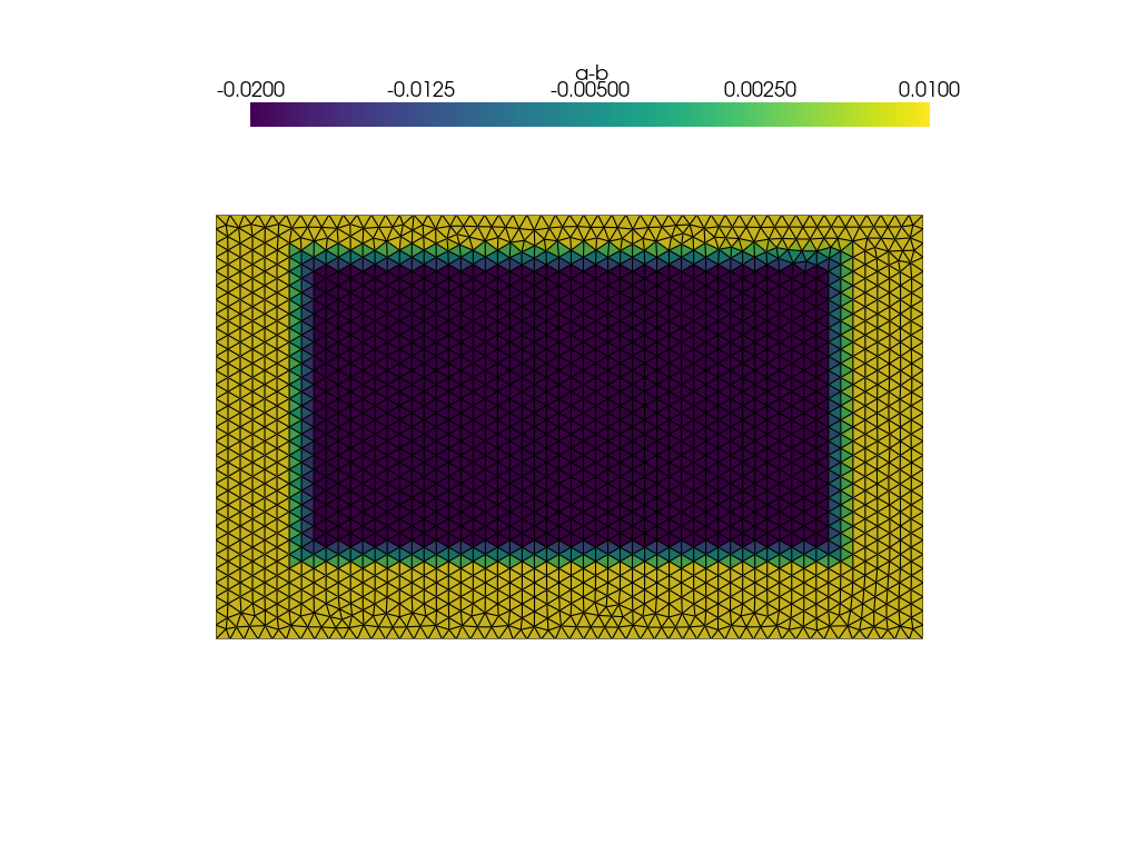
Fig. 5 Figure 1:mesh model and spatial distribution of a-b.
Step 2: calculate greenfunctions,we encapsulate all calculations in a class QDsim The Green function calculation is saved in the Corefunc directory defined in parameter.txt. The next time you start the program, you no longer need to calculate the Green function.
Step 3: Calculating Qusi-Dynamic model by loop
 start_time=time.time()

 totaloutputsteps=int(sim0.Para0['totaloutputsteps'])
 directory='outvtk'
 if not os.path.exists(directory):
     os.mkdir(directory)

 f=open('state.txt','w')
 f.write('iteration time_step(s) maximum_slip1_rate(m/s) maximum_slip2_rate(m/s) time(s) time(h)\n')

 if(sim0.useGPU==False):  #CPU case
     for i in range(totaloutputsteps):


         if(i==0):
             dttry=sim0.htry
         else:
             dttry=dtnext
         dttry,dtnext=sim0.simu_forward(dttry)
         year=sim0.time/3600/24/365
         if(i%10==0):
             print('iteration:',i)
             print('dt:',dttry,' max_vel:',np.max(np.abs(sim0.slipv)),' Seconds:',sim0.time,'  Days:',sim0.time/3600/24,
                 'year',year)
             memory_info = process.memory_info()
             print(f"Memory usage: {memory_info.rss / (1024 ** 2)} MB")
         f.write('%d %f %.16e %.16e %f %f\n' %(i,dttry,np.max(np.abs(sim0.slipv1)),np.max(np.abs(sim0.slipv2)),sim0.time,sim0.time/3600.0/24.0))


         if(sim0.Para0['outputvtk']=='True'):
             outsteps=int(sim0.Para0['outsteps']) #output steps
             if(i%outsteps==0):
                 fname=directory+'/step'+str(i)+'.vtk'
                 sim0.ouputVTK(fname)

 end_time = time.time()
 timetake=end_time-start_time
 f.write('Program end time: %s\n'%str(datetime.now()))
 f.write("Time taken: %.2f seconds\n"%timetake)

 print('Program end time: %s\n'%str(datetime.now()))
 print("Time taken: %.2f seconds\n"%timetake)
Step 4: Visualize Results
The simulation generates VTK files, visualize them using PyVista. You can also output all results in your own format by accessing the member variables of sim0 (e.g. sim0.slip).
 import pyvista as pv
 import glob
 import os

 # set vtk file path
 folder_path = "outvtk/"

 vtk_files = glob.glob(os.path.join(folder_path, "*.vtk")) + glob.glob(os.path.join(folder_path, "*.vtu"))


 #read state file for time show
 def is_number(s):
     try:
         float(s)
         return True
     except ValueError:
         return False

 def readstate(fname):
     f=open(fname,'r')
     K=0
     data0=[]
     for line in f:
         tem=line.split()

         if(len(tem)==6 and is_number(tem[0])==True):
             data0.append(np.array(tem).astype(float))
     return np.array(data0)
 state=readstate('state.txt')
 print(state.shape)

 # # show one figure
 plotter = pv.Plotter(off_screen=True)
 mesh = pv.read(vtk_files[10])
 slip_velocity = mesh['Slipv[m/s]']
 # Apply logarithmic transformation (e.g., base 10)
 # Add small constant (e.g., 1e-10) to avoid log(0) issues
 log_slip_velocity = np.log10(slip_velocity)

 # Assign the transformed scalars back to the mesh
 mesh['Log_Slipv[m/s]'] = log_slip_velocity
 scalar_range = (-12, 0)
 scalar_bar_args={
         'title': 'log10(slip rate)[m/s]',
         'position_x': 0.22,
         'position_y': 0.85,
     }
 plotter.add_mesh(mesh, scalars='Log_Slipv[m/s]', cmap="plasma", show_edges=True,clim=scalar_range,scalar_bar_args=scalar_bar_args)  # show shear stress

 #plotter.camera_position =[(0, -5, 0), (0, 0, 0), (0, 0, 1)]
 # plotter.add_scalar_bar(
 #         title='log10(Slip rate)[m/s]',  # Label for the colorbar
 #         position_x=0.25,         # Horizontal position (0 to 1, 0.25 centers it with width=0.5)
 #         position_y=0.05,         # Vertical position (close to bottom)
 #         width=0.5,              # Width of the colorbar (0 to 1, relative to plot)
 #         height=0.1,             # Height of the colorbar
 #         vertical=False          # Horizontal orientation
 #     )
 plotter.show(cpos='xz')

 # create animation
 outsteps=int(sim0.Para0['outsteps'])
 plotter = pv.Plotter(off_screen=True)
 plotter.open_gif('animation.gif')  # Initialize GIF output

 for i, vtk_file in enumerate(vtk_files):
     if(i*outsteps<len(state)):
         mesh = pv.read(folder_path+'step'+str(i*outsteps)+'.vtk')
         slip_velocity = mesh['Slipv[m/s]']
         # Apply logarithmic transformation (e.g., base 10)
         # Add small constant (e.g., 1e-10) to avoid log(0) issues
         log_slip_velocity = np.log10(slip_velocity)

         # Assign the transformed scalars back to the mesh
         mesh['Log_Slipv[m/s]'] = log_slip_velocity
         plotter.clear()  # Clear previous mesh
         plotter.add_mesh(
             mesh,
             scalars='Log_Slipv[m/s]',
             cmap="plasma",
             show_edges=False,
             clim=scalar_range,
             scalar_bar_args=scalar_bar_args
         )

         timeyear=state[i*outsteps,-1]/365
         plotter.add_text(f"Time: {timeyear:.8f} yr", position="upper_left", font_size=14, color="white", shadow=True)
         plotter.camera_position = 'xz'
         plotter.write_frame()  # Write frame to GIF

 plotter.close()
 print('Video has been saved.')
output:
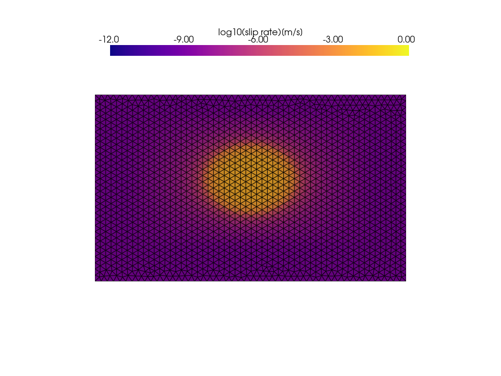
Fig. 6 Figure 2: Snapshot of slip rate.
GPU acceleration
Install cupy if you want to use GPU acceleration, we recommened to use conda in prompt terminal (e.g. CUDA 11.8):
conda install -c conda-forge cupy cudatoolkit=11.8
Note
CuPy relies on NVIDIA CUDA for GPU computing, so the following components are required:
NVIDIA GPU Driver: Ensure your system has a CUDA-capable NVIDIA GPU (check compatibility at https://developer.nvidia.com/cuda-gpus). The driver version must support the CUDA Toolkit version used by CuPy (e.g., CUDA 10.2–12.x for CuPy v13.x).
CUDA Toolkit: CuPy supports specific CUDA versions (check the latest compatibility at https://docs.cupy.dev/en/stable/install.html). Common versions: CUDA 11.8 or 12.2 are widely used.
The GPU operates in a similar way to the CPU, only the output is converted to numpy each time. Reading model and parameters is the same as CPU.
Note
Make sure to set GPU:True in the parameter.txt
start_time=time.time()

totaloutputsteps=int(sim0.Para0['totaloutputsteps'])
directory='outvtk'
if not os.path.exists(directory):
    os.mkdir(directory)

f=open('state.txt','w')
f.write(
    'iteration time_step(s) maximum_slip1_rate(m/s) '
    'maximum_slip2_rate(m/s) time(s) time(h)\n'
)

if(sim0.useGPU==True):  # GPU case
    sim0.initGPUvariable()

    for i in range(totaloutputsteps):
        print('iteration:',i)
        if(i==0):
            dttry=sim0.htry
        else:
            dttry=dtnext
        dttry,dtnext=sim0.simu_forwardGPU(dttry)

        # transform form cupy to numpy data
        sim0.slipv1=sim0.slipv1_gpu.get()
        sim0.slipv2=sim0.slipv2_gpu.get()
        sim0.slipv=sim0.slipv_gpu.get()
        sim0.slip=sim0.slip_gpu.get()
        sim0.Tt1o=sim0.Tt1o_gpu.get()
        sim0.Tt2o=sim0.Tt2o_gpu.get()
        sim0.Tt=sim0.Tt_gpu.get()
        # sim0.state1=sim0.state1_gpu.get()
        # sim0.state2=sim0.state2_gpu.get()
        sim0.rake=sim0.rake_gpu.get()

        year=sim0.time/3600/24/365
        if(i%10==0):
            print(
                'dt:',dttry,
                ' Seconds:',sim0.time,
                '  Days:',sim0.time/3600/24,
                'year',year
            )
            print(
                ' max_vel1:',np.max(np.abs(sim0.slipv1)),
                ' max_vel2:',np.max(np.abs(sim0.slipv2)),
                ' min_Tt1:',np.min(sim0.Tt1o),
                ' min_Tt2:',np.min(sim0.Tt2o)
            )

        f.write(
            '%d %f %.16e %.16e %f %f\n'
            %(
                i,
                dttry,
                np.max(np.abs(sim0.slipv1)),
                np.max(np.abs(sim0.slipv2)),
                sim0.time,
                sim0.time/3600.0/24.0
            )
        )

        memory_info = process.memory_info()
        print(f"Memory usage: {memory_info.rss / (1024 ** 2)} MB")

        if(sim0.Para0['outputvtk']=='True'):
            outsteps=int(sim0.Para0['outsteps'])  # output steps
            if(i%outsteps==0):
                fname=directory+'/step'+str(i)+'.vtk'
                sim0.ouputVTK(fname)
MPI-Based Execution on Linux
Step 1: Set Up Conda environment
Download latest Miniconda3, type:
wget https://repo.anaconda.com/miniconda/Miniconda3-latest-Linux-x86_64.sh -O miniconda.shIf you use iOS system, using following instead:
curl -o miniconda.sh https://repo.anaconda.com/miniconda/Miniconda3-latest-Linux-x86_64.shInstall Miniconda with the following command:
bash miniconda.sh -b -u -p ~/miniconda3Parameters:
-b: Batch mode, automatically accepts the license agreement.-u: Updates the installation if the directory already exists.-p ~/miniconda3: Specifies the installation directory (here, miniconda3 in the home directory).
After installation, initialize Conda for terminal use:
~/miniconda3/bin/conda initClose and reopen the terminal, or run:
source ~/.bashrcVerify the Installation, check the Conda version:
conda --versionAfter installation, create a new environment:
conda create -n PyQuake3D python=3.12Activate the environment:
conda activate PyQuake3DInstall openmpi via conda:
conda install -c conda-forge openmpi
Note
Dependencies: Ensure wget is installed. If not, install it:
sudo apt install wget(For Ubuntu/Debian)sudo yum install wget(For CentOS/RHEL)
Step 2: Install PyQuake3D and C++ Dependencies
Download from https://github.com/Computational-Geophysics/PyQuake3D
Install an MPI implementation and g++ compiler (including gcc and other related tools). Common options are:
sudo apt updatesudo apt install g++sudo apt install openmpi-bin libopenmpi-dev
Install PyQuake3D using pip:
pip install -e .(make sure PyQuake3D environment is activated).
Navigate to the
srcdirectory, runmaketo buildTDstressFS_C.so. The generated library is called by the Python scriptHmatrix.pyvia dynamic loading (e.g., usingctypes).
Note
MPI-CPU version is recommended for use on Linux because it requires compiling a C dynamic library, which is used for core function calculation acceleration. Compiling C dynamic libraries (DLLs) on Windows can be less convenient compared to Linux or other Unix-like systems for several reasons, stemming from differences in tooling, ecosystem, and system design. The MPI-CPU version includes all functions such as shear dilation, thermal pressurization, and lattice Hmatrice implementations.
Step 3: Examples for MPI-based backend
 import pyquake3d.readmsh as readmsh
 import numpy as np
 import sys
 import matplotlib.pyplot as plt
 import pyquake3d.QDsim as QDsim
 from math import *
 import time
 import argparse
 import os
 import psutil
 from datetime import datetime
 from mpi4py import MPI
 import pyquake3d.config as config
 import pyquake3d.Hmatrix as Hmat

 #Limit threads to 1 to avoid performance issues or resource conflicts caused by multi-threaded parallelism.
 os.environ["OMP_NUM_THREADS"] = "1"
 os.environ["MKL_NUM_THREADS"] = "1"
 os.environ["OPENBLAS_NUM_THREADS"] = "1"

 file_name = sys.argv[0]
 print(file_name)

 from config import comm, rank, size

 import sys

 if __name__ == "__main__":
     sim0=None
     fnamePara=None
     HMobj=None

     if(rank==0):
         print('# ----------------------------------------------------------------------------')
         print('# PyQuake3D: Boundary Element Method to simulate sequences of earthquakes and aseismic slips')
         print('# * 3D non-planar quasi-dynamic earthquake cycle simulations')
         print('# * Support for Hierarchical matrix compressed storage and calculation')
         print(f'# * Parallelized with MPI ({size} cpus)')
         print('# * Support for rate-and-state aging friction laws')
         print('# * Supports output to VTU formats')
         print('# * ----------------------------------------------------------------------------')
         try:

             parser = argparse.ArgumentParser(description="Process some files and enter interactive mode.")
             parser.add_argument('-g', '--inputgeo', required=True, help='Input msh geometry file to execute')
             parser.add_argument('-p', '--inputpara', required=True, help='Input parameter file to process')

             args = parser.parse_args()

             fnamegeo = args.inputgeo
             fnamePara = args.inputpara

         except:
             fnamegeo='examples/WMF/WMF20251203.msh'
             fnamePara='examples/WMF/parameter.txt'


         print('Input msh geometry file:',fnamegeo, flush=True)
         print('Input parameter file:',fnamePara, flush=True)

         nodelst,elelst=readmsh.read_mshV2(fnamegeo)                             #load mesh file
         Para=config.readPara(fnamePara)                                         #load parameter file
         sim0=QDsim.QDsim(elelst,nodelst,Para)                                   #create earthquake cycle model class
         HMobj=Hmat.Hmatrix(sim0.xg,sim0.nodelst,sim0.elelst,sim0.eleVec,Para)   #create Hmatrice class
         # output intial results
         # sim0.read_vtk('out_vtk/step450.vtu')                                  #load initial file from previous results
         fname='Init.vtu'
         sim0.writeVTU(fname,init=True)                                          #Output initial state


     HMobj = comm.bcast(HMobj, root=0)                                           #broadcast Hmatrice class
     sim0 = comm.bcast(sim0, root=0)                                             #broadcast Hmatrice class


     sim0.deploy_Hmatrix(HMobj)                                                  #deploy Hmatrice class


     sim0.calc_greenfuncs_mpi()                                                  #calculate core functions

     sim0.start()                                                                #Start forward simulation
MPI parallel running:
For large-scale simulations using the MPI-parallel H-matrix version, use the following command (not necessary in the root directory):
mpirun -n <N> python -m pyquake3d.main_mpi -g <input_geometry_file> -p <input_parameter_file>
For example, using 10 parallel mpi processes on BP5-QD model:
mpirun-np 10 python -m pyquake3d.main_mpi -g examples/BP5-QD/bp5t.msh-p examples/BP5-QD/parameter.txt
MPI-Based multi-GPU Execution on Linux
First, ensure that you have CUDA correctly installed. Please refer to the GPU acceleration section for detailed instructions.
The startup process for multi-MPI-based multi-GPU versions is basically the same as that for MPI-based CPU versions,
but with the following differences:the parameters in parameter.txt must ensure GPU:True,
and the number of GPU_cores must not be less than the number of CPU processes. You don’t need to specify the
Max thread workers and Batch_size, as it is only used by the single CPU/GPU version.
For MPI-Based multi-GPU version, use the following command (not necessary in the root directory):
mpirun -n <N> python -m pyquake3d.main_gpu_mpi -g <input_geometry_file> -p <input_parameter_file>
For example, using 10 parallel mpi processes on BP5-QD model:
mpirun-np 10 python -m pyquake3d.main_gpu_mpi -g examples/BP5-QD/bp5t.msh-p examples/BP5-QD/parameter.txt
Note
Memory Overhead: To run H-Matrix on a GPU, matrices and vectors must be flattened. The MPI-GPU version requires at least twice the memory of the CPU version due to repeated vector elements.
VRAM Allocation: Please verify your GPU’s VRAM capacity before starting. PyQuake3D automatically balances the memory load across all detected GPUs to minimize the risk of overflow.
Compatibility: PyQuake3D fully supports both multi-GPU and single-GPU acceleration.
The MPI-based multi-GPU version does not utilize GPU acceleration for fluid-related calculations, but this part of the code is still usable.
Post-Processing
Visualization
Results vtu files in dir out_vtu can be visualized with PyVista and Paraview. We provide the pyquake_tools code package, which is useful for visualizing the results of PyQuake3D, including plotting slip rate, stress, and other variables, as well as creating animations. You don’t need to install it, just copy the code in pyquake_tools to your working directory and import it in your script.
Simulation time
Basic information such as time and step size, as well as the maximum slip rate, is contained in state.txt to monitor whether the simulation results are normal and to visualize the simulation time.
The total number of rows in state.txt equals the number of the time steps.Each column is as follows:
iteration time_step(s) maximum_strike_slip_rate(m/s) maximum_dip_slip_rate(m/s) time(s) time(d)